Practical Methods for Real World Control Systems

ACC 2024 is in-person, and so this workshop will be in-person.

In-Person:  Tuesday, July 9, 2024, 8:30am to 5:30pm, Eastern Standard Time (EST)

No need to register for the conference to attend the workshop.

15 minute Intro Video about Workshop (from 2020)

Printable version of this flyer

Workshop Registration at ACC 2024 (through PaperPlaza) 

Presenters: Daniel Abramovitch, Sean Andersson, and Craig Buhr

Rationale:   The proverbial “gap” between control theory and practice has been discussed since the 1960s, but it shows no signs of being any smaller today than it was back then.  Despite this, the growing ubiquity of powerful and inexpensive computation platforms, of sensors, actuators and small devices, the “Internet of Things”, of automated vehicles and quadcopter drones, means that there is an exploding application of control in the world.  Any material that allows controls researchers to more readily apply their work and/or allows practitioners to improve their devices through best practices consistent with well understood theory, should be a good contribution to both the controls community and the users of control.  This workshop is intended as a small but useful step in that direction.

Prerequisite skills (of participants):     Undergraduate level knowledge of feedback systems, sampled data systems, and programming.  An honest interest in being able to translate control theory into physical control systems.

Intended Audience:          

We believe that this workshop will be of great interest to three types of audience members:

1) Academic researchers who are well versed in control theory but would like to learn more about issues practicing control engineers often encounter as well as techniques and methods often used outside of standard textbook solutions to enhance their students’ experience in the classroom and laboratory.

2) Practicing engineers who work on physical control systems and products that use control with an interest in connecting their work to “best practices” motivated by theory.

3) Students who may be interested in adding laboratory experiments to their research or want to know how to make what they have learned applicable in industry.

For each of these groups – and those that are somewhere in the intersection of them – this workshop will address the gap from both sides, so as to give the participant a more complete understanding of how it applies to their particular situation.

Topic overview:

The general style for each topic will be to present the issue, discuss rational ways of thinking about a solution, and where possible, show a demo to illustrate the idea.

· Overview, a.k.a. “Mind the Gap.” (8:30 am [30 min])

We will frame the workshop by taking a walk around a “practical” control loop, pausing to consider each element in a first-pass to set up the rest of the day.
[A companion document for the introduction can be found here.]

· System Models and Characterizing Them with Measurements, or why it’s both important and annoying to be discrete. (9:00 am [60 min])

Beginning with simple models, we will look at discretization and identification, exploring what a step response can tell us and when frequency methods are needed.

· Simple Controllers for Simple Models, or why so many controllers are PIDs, and why some are not. (10 am [90 min, including coffee break])

The choice of PID control is intimately related to what we can measure and model. We will explore this connection and look at how to tune your controllers and how to tweak them to get the most from their simple form.

· Practical Loop Design, Or Why Most Open Loops Should Be an Integrator, and How to Get There (11:30 am [30 min])

Here we will dive into loop shaping, including straightforward steps for loop shaping on a well instrumented system.  We also introduce Bode’s Integral Theorem and Stein’s Dirt Digging to understand the effects of loop shaping on closed-loop sensitivity.

· Resonances, Anti-Resonances, Filtering, and Equalization (12:00 pm [120 min, including 1 hour lunch break])

Simple models are good but reality often introduces additional complexity that must be dealt with. Here we will discuss filter shapes, structured, and programming used for loop shaping.

· Lunch (12:30 pm [60 min])

· Signal Detection, Sensors, Sample Rates, and Noise (Oh My!) (2 pm [90 min, including coffee break])

Returning to Bode’s Theorem, we will discuss how to get to noise sources so that we can minimize them at the source, before they get into the loop.  We will then discuss different types of filters that might be used to minimize noise at the source, including coherent demodulation for modulated sensor signals.

· Integrating in Feedforward Control (3:30 pm [30 min])

Feedforward control can make a controller better, if it’s done right. In this section we’ll explore the basic structures and uses of feedforward, and how to integrate feedforward into your setup.

· Ask Your Doctor: Is State Space Right for You?  (4 pm [30 min])

State space control has many advantages and yet is rarely used in practice. In this section we will try to understand why, and show a structure that may make it easier to apply.

· Pick a Chip, Any Chip: Or why real-time programming is too important to leave to folks who only know programming. (4:30 pm [30 min])

In the end, your controller has to be implemented on hardware. Here we will discuss some of those hardware choices and what it means for what you can do (and how you can do it).

· Closing Thoughts/Discussion (5 pm [30 min])

Yeah, cause everyone needs to summarize, right?

Workshop outline, topic details, and tentative schedule:

We expect that there will be more written material for the workshop than can be presented in a single day.  Any one of these topic areas could fill up half a day.  However, these are the areas we hope to illustrate in the time we have.

1. Overview (30 min)

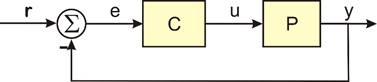
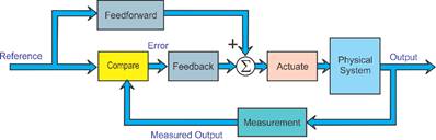
This will frame the style and topics of the workshop.  Control engineers will all recognize the block diagram above, but in going from that to implementation, we need to consider a much richer block diagram, a version of which is shown below.

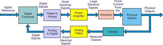
If we take a “walk around the loop” in this diagram, we discover a large set of pieces that need to be “gotten right” in order for the physical system to be properly controlled.  Often, these blocks have not been discussed since the second week of the first undergraduate controls class.    Specifically, we will first visit:

· The walk around the loop with a pure feedback loop, and with a feedback/feedforward loop.  How and when do we choose to add in feedforward components?  When can we not do this?  This ties into basic questions about the physical problem, what information is available, and what can be done with that information.

· Physics and modeling, and modeling that we can use.  How do we get from first principles (science) to models that help us do better control designs?  What parts of our models can we verify from actual measurements?  How do we work knowledge of current working loops into modeling for improved performance of the same system?

· Realizing that most modern implementations are on digital computers, how do we reconcile thinking in analog while implementing in digital?  When is “sampling fast” sufficient and what insights and improvements can we gain from paying attention to how we discretize things?

· Time constants, physical systems, and the controls that they push.  Process control, motion control, PLL (phase control and synchronization), mechatronic systems and other things that vibrate.

This introduction will introduce, frame, and motivate what we will do in the rest of the session, so while the topics are deep, they are intended as a “first pass” for the topics that will be more deeply discussed in the remaining sessions.

2. System Models and Characterizing Them with Measurements (60 min)

While advanced research often starts with some complex model, most practical control systems are based on an explicit or more often an implicit simple, low order, model.  In this segment, we will start by calling out these basic implicit models, discussing the systems that motivate and demonstrate them, and discuss what measurements can be made on such models.

We must accept that all of our measurements will be made in discrete time, and so our derived models must deal with the effects of sampling.  At the same time, we will show simple examples of why conventional discrete-time models can obscure the physical intuition of the original system so as to make tuning to physical parameter changes next to impossible for many systems.  A few simple examples will make this obvious and motivate the rest of the measurement and modeling discussion. Specific topics will include the following.

· The assumptions and limitations of time-domain identification on discrete-time models.

· First and second order system models, and where to find them.

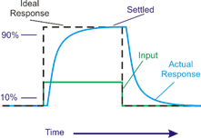
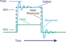
· Step response methods.  Using the simple models above, what can we hope to gain from a step response method?  How do we implement them in our control software so as to not be embarrassed by the better results from the digital oscilloscope?  What are the limitations of step response methods?  When is a step response measurement the only game in town?

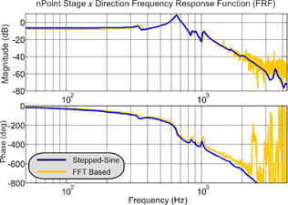
· Frequency response methods.   When are they better than step response?  When are they necessary in model characterization? When can you actually do such a measurement?  What are the tradeoffs between FFT frequency response methods and stepped sine (known as swept-sine in industry)? 

· Specialty instruments: Dynamic Signal Analyzers

· Curve fitting for frequency responses

· Effects of delays (NMP from Padé) and what it means for design

· Demo: MathWorks System Identification Toolbox

3. Simple Controllers for Simple Models (or why so many controllers are PIDs)  (90 minutes, with coffee break)

While PID controllers are the “Brand X” of most control Ph.D. candidates’ theses and spent the 1990s being derided by the denizens of fuzzy control, they remain today the most ubiquitous example of feedback controller design, by some measures accounting for 97% of all controllers in the field.  Rather than dismissing this as an alternative and boring reality, we will examine the underlying implicit assumptions about modeling the physical system – and how those models derive from what can be measured (from the previous segment), to motivate the generic and fundamental utility of PID controllers.  With that context, we will show in the first half of this segment:

· A unified framework for discussing PID controllers, which is helpful not only in generating a design, but also in understanding the underlying structures of off-the-shelf, commercial PID controllers. How do PID controllers relate to lead/lag controllers?

· A discussion for representing PID controllers in discrete time without losing the intuition of the continuous time framework.

· How PID controllers can be expected to behave in closed-loop for various low order models.

After the break, we will delve into some more advanced topics for PID controllers, as well as some demonstration of CACSD tools and physical examples:

· Tuning PID controllers:  from step response, from frequency response, from Åström et. al.’s relay method, from generalized Zeigler-Nichols.

· A discussion of windup and anti-windup mitigation: why it’s needed and what options exist.

· Why using ‘D’ in PID often fails to improve performance and how to fix that. Where is ‘D’ most often beneficial?

· Some PID code examples.

· Simple tweaks to PID structures to improve control (Prefiltering, PDF, proper structuring of PID for gain switching)

· Things to consider with the integrator depending on control goals.

· Demo: Matlab PID toolbox

· Tuning your PID using Control Systems Designer, PID tuner, and Auto-tuner

· Simulink PID block with anti-windup

4. Practical Loop Design, Or Why Most Open Loops Should Be a Constant or an Integrator, and How to Get There (30 minutes)

This section builds on the prior ones with a practical view of what is commonly called loop shaping.  The idea is to talk about how loop shaping affects practical stability margins (i.e. gain and phase margins) and how things that affect those margins affect the behavior of the closed-loop system.  With this context, we can discuss:

· Effects of dynamics, and how we can handle these with our filter equalizers.

· Desired open loop shapes (integrator) and closed-loop shapes (smooth low pass filter) and how they are related.

· Bringing it all together with Bode's Integral Theorem and Stein's Dirt Digging

5. Resonances, Anti-Resonances, Filtering, and Equalization (30  minutes + 60 minute lunch break + 30 minutes)

In the movie trailer, this section could be labeled, “when simple models go bad”.  Specifically, we will discuss system models with higher order dynamics, and what this means for control design.  In many frameworks, the first resonant mode signifies the frequency at which all control effort should stop. The commonly used PI controllers generally stop at ¼ the first resonant frequency.  For other systems, such as chemical process control, the performance limiting negative phase is dominated by delays in the system.  Getting beyond these limitations involve:

· Having a requirement to control faster.

· Having a reliable model of the higher frequency dynamics from measurements on the system itself. We will discuss ways to make these measurements more automated, more built in to the controller, thereby minimizing the per measurement costs.

· Having a design methodology for compensating for those dynamics.

With that as prelude, we will discuss filters in the context of loop design.

· Special Shapes; Notch, low-pass, band-pass, high-pass

· Special purpose filters:  median, rooftop, alpha-beta tracker, and complimentary filter

· Periodic averaging filter

· Filters as equalizers

· FIR and IIR filter blocks (C/Matlab code examples)

· Biquads and biquad cascades and why anyone should care

· Filters in control loops:  do’s and don’ts

· Illustration using simulation model of a motion control system that has a resonant peak. Show how notch filter + PID controller accomplishes much faster response than PID alone.

6. Signal Detection, Sensors, Sample Rates, and Noise (Oh My) (90 minutes)

In this section, we return to our prior discussion of filters, but now in the context of signal quality.  The pretexts are the input signals for our system, how they are detected, what the sensors and ADCs do to them, what determines sample rates, and how these affect our input signals and our control designs. We will briefly touch on:

· Using Bode’s Integral Theorem and Stein’s dirt digging to back out noise sources.

· Signal transducers for different systems.  You can’t hit what you can’t see and so a key and often neglected part of a control engineer’s toolkit is how to specify the right transducer for the job and where to put it.  What is available?  What are required sample rates versus what rates are supported by different measurement methods?  How is what you are asking of your control system bounded by your sensor and your computation?  Why are some fast ADCs so slow for control systems, and how do we choose?

· The limitations and risks of procuring ‘digital’ sensors off the shelf.

· Analog circuit filters, or do I really, really need to do that anti-alias stuff?

· Baseband vs. modulated signals:  Many inputs to control systems are modulated on some other signal.  Leaving detection of these to “the circuit folks” may severely limit our control loops.

7 Integrating in Feedforward Control (30 minutes)

This section will discuss practical application of feedforward control to a feedback loop.  In large part, feedforward can remove a lot of the potential error from the control loop, unburdening the feedback control system. But in some situations, it can introduce error.    There are two basic forms of FF: Plant Injection (PI) and Closed Loop Injection (CLI).

· When can we use feedforward? When is it a good idea?  What is the benefit?

· How should the feedback loop be designed for feedforward (idea: integrator OL -> LPF closed-loop -> multi-lead feedforward).  What about PI form?  How to choose.

· What do each of FF choices (PI and CLI) imply for feedback controller design?

· Using prefilters (shaping) to prevent overshoot

· Repetitive control and adaptive feedforward cancellers

· Feedforward control from auxiliary sensors

8. Ask Your Doctor: Is State Space Right for You? (30 minutes)

State space is the way to do things ‘right’ in academia and yet seems to have limited used use in industry, depending usually upon the size and expense of the system, and of course, the number of resonances that have to be dealt with.  To get industry folks to use SS, there has to be a clear set of advantages, and there has to be a clear path around the gotchas.  It has always been pitched as a way to handle MIMO systems, but many MIMO systems are really handled as a decoupled set of SISO systems.  To really make the case, we need to show the specific advantages of state space over transfer function methods in practical, ordinary SISO systems:

a) State space gives us a structural look inside the dynamics of a system having order > 2, beyond the ones that we can typically measure with sensors, and so the state space model should be realized in a way that the discrete form represents physical reality.

b) State space can allow us to build a model framework for things like missing samples in a system or integrating together multiple sensors of different rates and qualities.

c) State space can allow us to embed nonlinear relationships in the states that are more difficult to represent by transfer functions. These modifications are more often useful in modeling and simulation of the plant than in controls analysis, but perhaps useful as non-linear observers (estimators).

d) It should be emphasized that model based measurement and control depend upon ... a good model. 

e) How do we make State Space work on different classes of systems? The Biquad State Space structure will be discussed as an example.

9. Pick a Chip, Any Chip (30 minutes)

At some point, you need a work environment, an integrated hardware in the loop development platform.  Lots of work gets done on cheapo stuff.  At the same time, there are the higher end, "Matlab/NI will do the FPGA stuff for you" systems.  What are the tradeoffs, how does one choose, and eventually how does one implement control laws on a real system?  If it costs $10K to even get started with Matlab/NI and it costs $200 to work with a Raspberry Pi or Arduino, the choice is obvious if you don’t have a big bankroll to work with.  What are the tradeoffs and consequences? 

Similarly, we do not spend much time thinking about converter chips, ADCs and DACs, except for a cursory mumble about the number of bits and the sample rates.  Still, it makes little sense to specify a fast sample rate to reduce latency only to have a 15-sample period delay in the conversion pipeline and a slow, multiplexed, serial readout of the samples.  We will touch on this briefly.

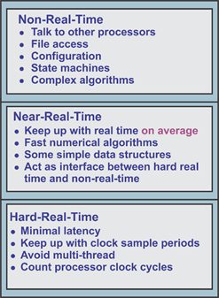
At the same time, few system engineers spend a large chunk of their time thinking about programming tools, styles, and models, relinquishing these areas to ‘other’ non- control people.  Not only does this make it harder for them to satisfy the system’s real-time requirements, but it also makes it more difficult for them to evaluate and acquire the right skills or people needed to complete the tasks. The issue is that different parts of an intelligent real-time system have different timing requirements and this means that each of these requirement sets lead to different programming models. We will discuss these in this section, as a guide to how system engineers can properly handle these issues.

· What different real-time systems are available? PIC, Arduino, Raspberry Pi, Zynq, Altera SoC, and a partridge in a pear tree.  How do we pick one? Bandwidth, noise, compilers? Hardware?  Legacy designs? 

· Demo: Deploying your Matlab-designed controller using:

o Simulink built-in support for Arduino, Lego, Raspberry Pi, and other low-cost hardware

o Embedded Coder

o HDL Coder

Presenters’ short bios:

· Dr. Daniel Abramovitch (Agilent Technologies)

Danny Abramovitch earned degrees in Electrical Engineering from Clemson (BS) and Stanford (MS and Ph.D.), doing his doctoral work under the direction of Gene Franklin. Upon graduation, and after a brief stay at Ford Aerospace, he accepted a job at Hewlett-Packard Labs, working on control issues for optical and magnetic disk drives for 11 1/2 years.  He moved to Agilent Laboratories shortly after the spinoff from Hewlett-Packard, where he has spent 24 years working on test and measurement systems.  He is currently in Agilent’s Mass Spectrometry Division working on improved real-time computational architectures for Agilent’s mass spectrometers, including the new Ultivo Tandem Quad product.

Danny is a Fellow of the IEEE and the recipient of the American Automatic Control Council’s 2024 Babatunde Ogunnaike Control Practice Award. He was Vice Chair for Industry and Applications for the 2004 American Control Conference (ACC) in Boston, for the 2009 ACC in St. Louis, and the 2022 ACC in Atlanta.  He was Vice Chair for Workshops at the 2006 ACC in Minneapolis and the 2024 ACC in Atlanta, and for Special Sessions at the 2007 ACC in New York. He was Program Chair for the 2013 ACC and is General Chair of the recent 2016 ACC in Boston. He has helped organize conference tutorial sessions on topics as varied as disk drives, atomic force microscopes, phase-locked loops, laser interferometry, and how business models and mechanics affect control design. He served as the Chair of the IEEE CSS History Committee from 2001 to 2010.  Danny is credited with the original idea for the clocking mechanism behind the DVD+RW optical disk format and is co-inventor on the fundamental patent.  He was on the team that prototyped Agilent’s first 40Gbps Bit Error Rate Tester (BERT) and was able to cite a Douglas Adams book in one of his patents relating to that device.  Along with his co-author, Gene Franklin, he was awarded the 2003 IEEE Control Systems Magazine Outstanding Paper Award. His favorite paper remains the one prompted by a question from his then 3-year-old son, which showed that the outrigger was a feedback mechanism that predated the water clock by at least a 1000 years. He will be a plenary speaker at the 2024 IFAC Conference on Advances in PID Control in Spain. He was a Keynote Lecturer at the 2015 Multi-Conference on Decision and Control in Sydney, Australia, a Plenary Lecturer at the 2020 Conference on Control Technology and Automation in Montreal, and a Semi-Plenary speaker at the inaugural Modeling, Estimation, and Control Conference in Austin.  His recent work for Agilent was on future atomic force microscopes and high precision interferometers.  His current work involves improving the real-time data collection and signal processing on Agilent’s Mass Spectrometers, and is part of the team that created Agilent’s multi-award winning Ultivo Tandem Quad LC Mass Spectrometer. He is the holder of over 20 patents and has published nearly 50 reviewed technical papers.

· Professor Sean Andersson (Boston University)

Sean B. Andersson received the B.S. degree in engineering and applied physics from Cornell University, Ithaca, NY, USA, in 1994, the M.S. degree in mechanical engineering from Stanford University, Stanford, CA, USA, in 1995, and the Ph.D. degree in electrical and computer engineering from the University of Maryland, College Park, MD, USA, in 2003. He has worked at AlliedSignal Aerospace and Aerovironment, Inc. and is currently an Associate Professor of mechanical engineering and of systems engineering with Boston University, Boston, MA, USA. His research interests include systems and control theory with applications in scanning probe microscopy, dynamics in molecular systems, and robotics. He received an NSF CAREER award in 2009, is a senior member of the IEEE, and has been an associate editor for the IEEE Transactions on Automatic Control since 2014 and for the SIAM Journal on Control and Optimization since 2013. He has served as the Exhibitions Chair for the 2013 American Control Conference (ACC) in Washington D.C. and as the Local Arrangements Chair for the 2016 ACC in Boston.

· Dr. Craig Buhr (Mathworks)

Craig Buhr received his B.S., M.S. and Ph.D. from the School of Mechanical Engineering at Purdue University. He joined MathWorks in 2003 as a Senior Developer for the Controls and Identification products. He currently manages the Control Design development team, whose focus is developing tools for the design and analysis of control systems.  His research interests include dynamic system modelling, control theory and computer aided control system design.