Practical Methods for Real World Control Systems

A half-day workshop, preceding IFAC Mechatronics & MoVic 2022. 

Tuesday, September 6, 2022, 1pm to 5:00pm, Pacific Standard Time (PST, GMT-7)

This workshop is in person at UCLA preceding the conference.

15 Minute Invite/Intro Video About Workshop

Printable version of this flyer

Workshop registration at MSMVC 2022 (PaperCept) 

(Select MSMVC 2022.  You will need a free PaperCept PIN. You do not need to be registered for the conference to register for the workshop.  However, the registration will ask you to state your conference registration category.  The main thing is to specify academic/professional or student/retiree. On the next page you will be given the option to register for the conference and workshops or just the workshops.)

Presenter: Daniel Abramovitch

Rationale:   The proverbial “gap” between control theory and practice has been discussed since the 1960s, but it shows no signs of being any smaller today than it was back then.  Despite this, the growing ubiquity of powerful and inexpensive computation platforms, of sensors, actuators and small devices, the “Internet of Things”, of automated vehicles and quadcopter drones, means that there is an exploding application of control in the world.  Any material that allows controls researchers to more readily apply their work and/or allows practitioners to improve their devices through best practices consistent with well understood theory, should be a good contribution to both the controls community and the users of control.  This workshop is intended as a small but useful step in that direction.

Prerequisite skills (of participants):     Undergraduate level knowledge of feedback systems, sampled data systems, and programming.  An honest interest in being able to translate control theory into physical control systems.

Intended Audience:          

We believe that this workshop will be of great interest to three types of audience members:

1) Academic researchers who are well versed in control theory but would like to learn more about issues practicing control engineers often encounter as well as techniques and methods often used outside of standard textbook solutions to enhance their students’ experience in the classroom and laboratory.

2) Practicing engineers who work on physical control systems and products that use control with an interest in connecting their work to “best practices” motivated by theory.

3) Students who may be interested in adding laboratory experiments to their research or want to know how to make what they have learned applicable in industry.

For each of these groups – and those that are somewhere in the intersection of them – this workshop will address the gap from both sides, so as to give the participant a more complete understanding of how it applies to their particular situation.

Topic overview:

The general style for each topic will be to present the issue, discuss rational ways of thinking about a solution, and where possible, show a demo to illustrate the idea.

· Overview, a.k.a. “Mind the Gap.” (1:00 pm [20 min])

We will frame the workshop by taking a walk around a “practical” control loop, pausing to consider each element in a first-pass to set up the rest of the workshop.

· System Models and Characterizing Them with Measurements, or why it’s both important and annoying to be discrete. (1:20 pm [40 min])

Beginning with simple models, we will look at discretization and identification, exploring what a step response can tell us and when frequency methods are needed.

· Simple Controllers for Simple Models, or why so many controllers are PIDs, and why some are not. (2 pm [60 min])

The choice of PID control is intimately related to what we can measure and model. We will explore this connection and look at how to tune your controllers and how to tweak them to get the most from their simple form.

· Coffee/Bio Break (3 pm [15 min])

· Practical Loop Design, Or Why Most Open Loops Should Be an Integrator, and How to Get There (3:15 pm [30 min])

Here we will dive into loop shaping, including straightforward steps for loop shaping on a well instrumented system.  We also introduce Bode’s Integral Theorem and Stein’s Dirt Digging to understand the effects of loop shaping on closed-loop sensitivity.  We will also mention some of the implementation details that often limit this.

· Filtering and Equalization for Mechatronic Systems and How to Actually Make State Space Useful for Them (3:45 pm [45 min])

If everything could be handled with a PID, the world would be a much stiffer place.  In order to get to that ideal open loop, we need to filter in an intelligent way.  Along the path, someone may mention state space.  We will try to understand why this is so rare in mechatronic systems and introduce a structure that may change that.

· Integrating in Feedforward Control (4:30 pm [30 min])

Feedforward control can make a controller better, if it’s done right. In this section we’ll explore the basic structures and uses of feedforward, and how to integrate feedforward into your setup.

Workshop outline, topic details, and tentative schedule:

We expect that there will be more written material for the workshop than can be presented in a half day.  Any one of these topic areas could fill up half a day.  However, these are the areas we hope to illustrate in the time we have.

1. Overview (20 min)

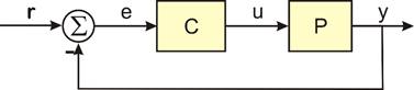
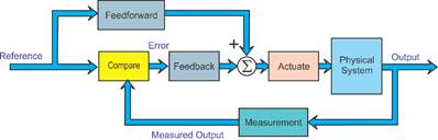
This will frame the style and topics of the workshop.  Control engineers will all recognize the block diagram above, but in going from that to implementation, we need to consider a much richer block diagram, a version of which is shown below.

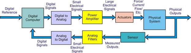
If we take a “walk around the loop” in this diagram, we discover a large set of pieces that need to be “gotten right” in order for the physical system to be properly controlled.  Often, these blocks have not been discussed since the second week of the first undergraduate controls class.    Specifically, we will first visit:

· The walk around the loop with a pure feedback loop, and with a feedback/feedforward loop.  How and when do we choose to add in feedforward components?  When can we not do this?  This ties into basic questions about the physical problem, what information is available, and what can be done with that information.

· Physics and modeling, and modeling that we can use.  How do we get from first principles (science) to models that help us do better control designs?  What parts of our models can we verify from actual measurements?  How do we work knowledge of current working loops into modeling for improved performance of the same system?

· Realizing that most modern implementations are on digital computers, how do we reconcile thinking in analog while implementing in digital?  When is “sampling fast” sufficient and what insights and improvements can we gain from paying attention to how we discretize things?

· Time constants, physical systems, and the controls that they push.  Process control, motion control, PLL (phase control and synchronization), mechatronic systems and other things that vibrate.

This introduction will introduce, frame, and motivate what we will do in the rest of the session, so while the topics are deep, they are intended as a “first pass” for the topics that will be more deeply discussed in the remaining sessions.

2. System Models and Characterizing Them with Measurements (40 min)

While advanced research often starts with some complex model, most practical control systems are based on an explicit or more often an implicit simple, low order, model.  In this segment, we will start by calling out these basic implicit models, discussing the systems that motivate and demonstrate them, and discuss what measurements can be made on such models.

We must accept that all of our measurements will be made in discrete time, and so our derived models must deal with the effects of sampling.  At the same time, we will show simple examples of why conventional discrete-time models can obscure the physical intuition of the original system so as to make tuning to physical parameter changes next to impossible for many systems.  A few simple examples will make this obvious and motivate the rest of the measurement and modeling discussion. Specific topics will include the following.

· The assumptions and limitations of time-domain identification on discrete-time models.

· First and second order system models, and where to find them.

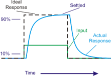
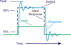
· Step response methods.  Using the simple models above, what can we hope to gain from a step response method?  How do we implement them in our control software so as to not be embarrassed by the better results from the digital oscilloscope?  What are the limitations of step response methods?  When is a step response measurement the only game in town?

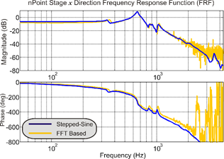
· Frequency response methods.   When are they better than step response?  When are they necessary in model characterization? When can you actually do such a measurement?  What are the tradeoffs between FFT frequency response methods and stepped sine (known as swept-sine in industry)? 

· Curve fitting for frequency responses

· Effects of delays (NMP from Padé) and what it means for design

3. Simple Controllers for Simple Models (or why so many controllers are PIDs)  (60 minutes)

While PID controllers are the “Brand X” of most control Ph.D. candidates’ theses and spent the 1990s being derided by the denizens of fuzzy control, they remain today the most ubiquitous example of feedback controller design, by some measures accounting for 97% of all controllers in the field.  Rather than dismissing this as an alternative and boring reality, we will examine the underlying implicit assumptions about modeling the physical system – and how those models derive from what can be measured (from the previous segment), to motivate the generic and fundamental utility of PID controllers.  With that context, we will show in the first half of this segment:

· A unified framework for discussing PID controllers, which is helpful not only in generating a design, but also in understanding the underlying structures of off-the-shelf, commercial PID controllers. How do PID controllers relate to lead/lag controllers?

· A discussion for representing PID controllers in discrete time without losing the intuition of the continuous time framework.

· How PID controllers can be expected to behave in closed-loop for various low order models.

· Tuning PID controllers:  from step response and from frequency response.

· Why using ‘D’ in PID often fails to improve performance and how to fix that. Where is ‘D’ most often beneficial?

· Things to consider with the integrator depending on control goals, including thoughts on integrator anti-windup.

4. Practical Loop Design, Or Why Most Open Loops Should Be a Constant or an Integrator, and How to Get There (30 minutes)

This section builds on the prior ones with a practical view of what is commonly called loop shaping.  The idea is to talk about how loop shaping affects practical stability margins (i.e. gain and phase margins) and how things that affect those margins affect the behavior of the closed-loop system.  With this context, we can discuss:

· Effects of dynamics, and how we can handle these with our filters as equalizers.

· Desired open loop shapes (integrator) and closed-loop shapes (smooth low pass filter) and how they are related.

· Bringing it all together with Bode's Integral Theorem and Stein's Dirt Digging

5. Filtering and Equalization for Mechatronic Systems and How to Actually Make State Space Useful for Them (45 minutes)

In the movie trailer, this section could be labeled, “when simple models go bad”.  Specifically, we will discuss system models with higher order dynamics, and what this means for control design.  In many frameworks, the first resonant mode signifies the frequency at which all control effort should stop. The commonly used PI controllers generally stop at ¼ the first resonant frequency.  For other systems, such as chemical process control, the performance limiting negative phase is dominated by delays in the system.  Getting beyond these limitations involve:

· Having a requirement to control faster.

· Having a reliable model of the higher frequency dynamics from measurements on the system itself. We will discuss ways to make these measurements more automated, more built in to the controller, thereby minimizing the per measurement costs.

· Having a design methodology for compensating for those dynamics. Filters as equalizers, and why mechatronic systems usually use biquad cascades.

· Filters in control loops:  do’s and don’ts

· Illustration using simulation model of a motion control system that has a resonant peak. Show how notch filter + PID controller accomplishes much faster response than PID alone.

With this framework, we will move to the “third rail” of mechatronic control of high Q systems.  We will discuss what makes this so hard and discuss how the Biquad State Space structure allows us to move beyond the typical limitations.   We will also show how the BSS restores some of the original promise of state space methods, allowing us to have digital models that more closely mirror our physical models, which in turn allows us to compare models with lab measurements – to put virtual and physical scope probes in corresponding parts of the model and physical system.

6. Integrating in Feedforward Control (30 minutes)

This section will discuss practical application of feedforward control to a feedback loop.  In large part, feedforward can remove a lot of the potential error from the control loop, unburdening the feedback control system. But in some situations, it can introduce error.    There are two basic forms of FF: Plant Injection (PI) and Closed Loop Injection (CLI).

· When can we use feedforward? When is it a good idea?  What is the benefit?

· How should the feedback loop be designed for feedforward (idea: integrator OL -> LPF closed-loop -> multi-lead feedforward).  What about PI form?  How to choose.

· What do each of FF choices (PI and CLI) imply for feedback controller design?

· Repetitive control and adaptive feedforward cancellers

· Feedforward control from auxiliary sensors

Presenter’s short bio:

· Dr. Daniel Abramovitch (Agilent Technologies)

Danny Abramovitch earned degrees in Electrical Engineering from Clemson (BS) and Stanford (MS and Ph.D.), doing his doctoral work under the direction of Gene Franklin. Upon graduation, and after a brief stay at Ford Aerospace, he accepted a job at Hewlett-Packard Labs, working on control issues for optical and magnetic disk drives for 11 1/2 years.  He moved to Agilent Laboratories shortly after the spinoff from Hewlett-Packard, where he has spent 19 years working on test and measurement systems.  He is currently in Agilent’s Mass Spectrometry Division working on improved real-time computational architectures for Agilent’s mass spectrometers, including the new Ultivo Tandem Quad product.

Danny is a Fellow of the IEEE and was Vice Chair for Industry and Applications for the 2004 American Control Conference (ACC) in Boston.  He was Vice Chair for Workshops at the 2006 ACC in Minneapolis and at the 2022 ACC in Atlanta, for Special Sessions at the 2007 ACC in New York, and for Industry and Applications for the 2009 ACC in St. Louis. He was Program Chair for the 2013 ACC and was General Chair of the recent 2016 ACC in Boston. He has helped organize conference tutorial sessions on topics as varied as disk drives, atomic force microscopes, phase-locked loops, laser interferometry, and how business models and mechanics affect control design. He served as the Chair of the IEEE CSS History Committee from 2001 to 2010.  Danny is credited with the original idea for the clocking mechanism behind the DVD+RW optical disk format and is co-inventor on the fundamental patent.  He was on the team that prototyped Agilent’s first 40Gbps Bit Error Rate Tester (BERT) and was able to cite a Douglas Adams book in one of his patents relating to that device.  Along with his co-author, Gene Franklin, he was awarded the 2003 IEEE Control Systems Magazine Outstanding Paper Award. His favorite paper remains the one prompted by a question from his then 3-year-old son, which showed that the outrigger was a feedback mechanism that predated the water clock by at least a 1000 years. He was a Keynote Lecturer at the 2015 Multi-Conference on Decision and Control in Sydney, Australia and a plenary speaker at the 2020 Conference on Control Technology and Applications (this conference).  His recent work for Agilent was on future atomic force microscopes and high precision interferometers.  His current work involves improving the real-time data collection and signal processing on Agilent’s Mass Spectrometers, and is part of the team that created Agilent’s multi-award winning Ultivo Tandem Quad LC Mass Spectrometer. He is the holder of over 20 patents and has published nearly 50 reviewed technical papers.